Fun with hypergeometric functions

Image from https://www.tetramode.com/collections/hypergeometry

Recently I was listening to a podcast where people play a role-playing game called Delta Green. Delta Green is set in a Lovecraftian universe. The players come up against the horrors of an uncaring universe, and hope their wits can carry the day. In this particular game, a set of mathematical concepts, referred to in the game as hypergeometric mathematics, was unfortunately acting as a beacon to entities antithetical to humanity.

This plotline got me to reminiscing about my grad school days. Why? Because I spent several years working with and studying something called hypergeometric functions. Yes, Lovecraft fans, there is such a thing in the real world. They are real and they are fascinating.

Delvers into hypergeometric mathematics draw their power from two real grimoires. As powerful and esoteric as the Eltdown Shards or the Book of Eibon, these are spoken of only in whispers in dark hallways; their names are difficult for the human vocal tract to pronounce. Those who dare speak their names out loud call these Abramowitz and Stegun, and Gradshteyn and Ryzhik. If you dare to follow the path I lay out here, and are willing to risk your very sanity, arm yourselves with these tomes!

I’ll show you a way to use hypergeometric functions to solve a problem in quantum mechanics. This problem describes how two parallel universes interfere with each other, and how our current Universe splits into both of them.

(If you would like to see more details, all of this is a summary of work I wrote up here in Chapter 4.1.5.)

A Warm Up

I was one of the founders of D-Wave. D-Wave builds quantum computers.

In the kind of quantum computer D-Wave builds, a textbook quantum problem ends up playing a central role in understanding what they do and how they work. This is called the Landau-Zener problem.

In the Landau-Zener problem, we want to calculate what the probability is of a quantum system ending up in different possible states after something has happened. You can think of these different states as corresponding to different Universes, differing only in the state of the quantum system in question.

Even though the Landau-Zener problem is one of the simplest problems in quantum mechanics, it exhibits many very interesting and highly non-trivial features.

In hindsight, thinking about this problem for many years was one of the reasons I felt (and still feel) that D-Wave made the right decision about what model of computation to back. Many people in the quantum information field don’t sufficiently understand what the solutions of this particular problem imply. In my view this has caused the field of quantum computing to be held back.

I’ll start by introducing the problem in its simplest, original incarnation. Note that what this post is ultimately about are solving different sorts of differential equations, so there will be math. I’ll try along the way to describe what the math is doing for us.

OK, let’s begin!

In physics there is a special matrix called the Hamiltonian. The eigenvalues of this matrix are the allowed energies of a system, and the eigenvectors are the allowed states of the system.

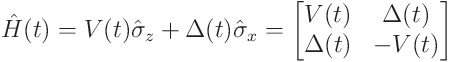
Here is the Hamiltonian of a two-level system (for example, a single qubit) under the influence of an external linear time-varying field. (The σ terms are 2x2 Pauli matrices.)

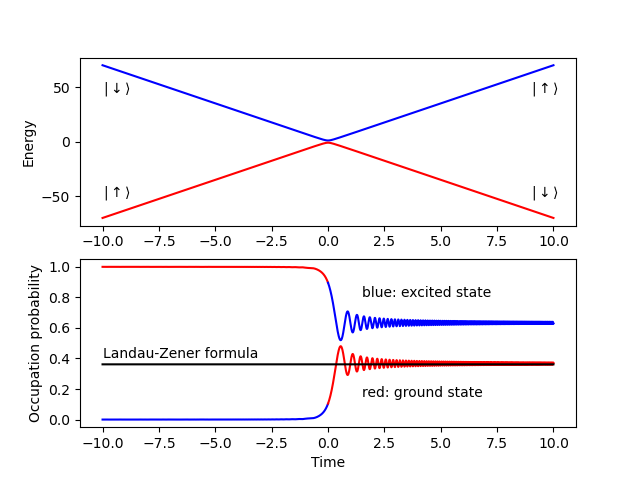
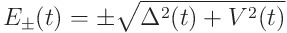
We can get the eigenvalues (allowed energies) by diagonalizing this 2x2 matrix. They are functions of time, because the matrix we are diagonalizing depends on time. Here they are, first as algebra and then as a picture.

The orange line is the negative energy branch (the ground state) and the blue line is the positive energy branch (the excited state). The red circle is meant to illustrate that we initialize the system in the ground state in the far past, and the red arrow indicates that we are sweeping forward in time (think of the red circle like a bead on a wire, moving left to right). In the far past, the “up” state of the qubit is the ground state, and the “down” state is the excited state. In the far future, the “up” state becomes the excited state and the “down” state becomes the ground state. If the qubit ends up where the green dot is, that means it ends up in the ground state. If however it ends up where the blue dot is, that’s the excited state. The Landau-Zener problem asks us to compute what the probabilities of ending up in these are. One interesting aside is that here we see one of the really fascinating aspects of quantum physics on display — how this system behaves is irreducibly probabilistic. While we can compute the probabilities (as we will see shortly), we can’t, even in principle, know for certain which of these two possibilities our qubit will end up in for any particular experiment.

The problem we want to solve is this. If we start this system at some time in the distant past (on the far left of the image where the red dot is) in the lower energy state, and we ‘sweep’ it from left to right, what is the probability it will still be in the lower energy state (where the green dot is) at some time in the distant future (on the far right of the image)?

(As an aside, if the system stays in its ground state throughout and ends up in the lower energy state, like a literal bead on a wire, that’s called an adiabatic transition. If it ‘skips’ up to the higher energy, like a record track skipping, that’s called a diabatic transition. The point where the higher and lower energies get closest is called an anti-crossing, and the difference between the two energy levels at that point is called the minimum energy gap.)

Here’s one way to solve this problem. If we plug the Hamiltonian above into the Schrodinger equation (using units where ℏ = 1)

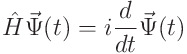
we get

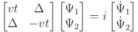
where overdots are derivatives with respect to time. Doing the matrix multiplication gives two equations:

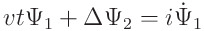
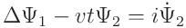
Eliminating variables allows us to write

These are differential equations with known analytic solutions, called parabolic cylinder functions. If we add in our desired initial condition (the system is in the lower energy state in the far past), and take the limit as t gets large, the probability of staying in the initial “up” state is

This is the probability of “skipping” up to the top state, which isn’t exactly what we asked for. But because probabilities have to sum to one, the answer to the problem we originally posed is just 1 minus that:

This is the solution to the simplest version of the Landau Zener problem! Here is a picture of the exact solutions for the transition probabilities over time, for one choice of parameters.

Top: Energy eigenvalues. Bottom: Occupation probabilities for the two states over time. I colored the lines to show that the top function is the probability of being “up”, which switches from being the low energy to high energy branch at t=0, and the bottom function is the probability of being “down”, which also switches. The Landau-Zener probability is the far future asymptote of the probability of being in the “correct” / ground state in the far future. This example used time in units of nanoseconds, v=7 GHz² and Δ=1 GHz.

A couple of observations about this:

1. The answer is irreducibly probabilistic. If you actually do this experiment, you cannot, even in principle, determine which of the two states you will end up in. All you can know are these probabilities.
2. The oscillatory behavior near & after the anticrossing is a signature of coherent quantum tunneling between two parallel universes, differing only in the state of the qubit. A way of thinking about this is near the anticrossing, Nature itself hasn’t figured out which of the two possibilities is most likely! It wavers between two different parallel Universes as the energies get closer to each other.
3. If Δ goes to zero, the probability of ending up in the ground state goes to zero exponentially.
4. The parameter v controls how fast we sweep through the transition. The slower you sweep, the more chance that you end up in the ground state. This is connected to something called the adiabatic theorem, which says that as long as Δ is not zero, if you make v small enough you can make the probability of remaining in the ground state arbitrarily close to 1. This observation was one of the inspirations for early work on the adiabatic model of quantum computation.

A lot is going on in this simple exactly solvable example!

The key to what we just did working is that when we got to the step where the wavefunction was written as a second order differential equation, it just so happened that that particular differential equation had a special function that solved it.

A Generalized Landau-Zener Problem

Let’s say we have something like the above problem, but generalized a bit. Specifically let’s use the Hamiltonian

You can check that this is a generalized version of the previous case. Here we have allowed energies

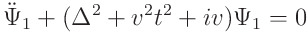
If we follow the exact same prescription as before, plugging this Hamiltonian into the Schrodinger equation and eliminating one of the variables, we get

Now unfortunately, for any old values of V and Δ, this differential equation doesn’t have nice exact closed form solutions like in the original simpler problem.

Prepare for … hypergeometric madness!!!

Here’s a cool trick. Let’s make a change of variables from t to some other function z(t), where the only requirement is that the map is 1–1 (for every time t there is a unique value of z(t)). The one we’ll use here is

If we rewrite our differential equation in terms of z instead of t, and indicate differentiation with respect to z with a prime, we get

OK … so that looks like a horrid mess. What did we gain? Well here’s the thing. There is a differential equation that looks a lot like this, called Riemann’s differential equation (RDE). And guess what functions are solutions to RDE? Hypergeometric functions!!!

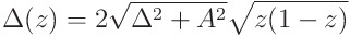
The thing above isn’t quite right yet. Let me show you two choices of V and Δ that map down to the RDE. First let’s choose

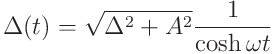
or equivalently as functions of z,

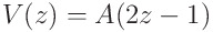
This models a scenario where we are sweeping an external bias field while the tunneling term is ‘pulsed’ on during the transition.

Sticking these into our equation gives

where

That, my friends, is a specific case of the RDE, and the wavefunction can now be written in terms of hypergeometric functions!!!

Here’s what the general solution looks like.

The F things are ₂F₁ (Gaussian) hypergeometric functions.

If we require that at z=0 (corresponding to the far past) the occupation probability is zero, we find that D=0. If we use some asymptotic behavior in the far future, we can then find C, which gives us the wavefunction at all times. Here it is:

If we take the far future limit (z approaching 1 which is the same as t going to infinity), we find that

This result is exact… and sort of weird. In the limit where A is small, the probability of making a transition oscillates from 0 to 1 as we change Δ. So you can make Δ smaller and increase the transition probability and vice versa!

Here’s a picture of what the transition probabilities look like for all time, for Δ=1, A=0.25 and ω=1.

For this case the physics is similar to the simple Landau-Zener case; coherent tunneling causes probability oscillations when the tunneling term is on, then stabilizing once it’s turned off.

You can do the exact same thing for the case where Δ is constant for all time and

as before. Going through the hypergeometric rigomarole, the answer for the transition probability is

What did we learn from all of this?

The Schrodinger equation is a differential equation, and sometimes the specific kind of differential equation it is has exact solutions.

If you spend many years of your life perusing the forbidden Abramowitz and Stegun and Gradshteyn and Ryzhik, you may find blasphemous recipes for (among other things) hypergeometric mathematics that can help you get exact closed form solutions to these, at the cost of having to make many, many sanity rolls.

Just for fun, I plotted the phase of the hypergeometric function in the first example above for part of the complex plane while randomly increasing both A₀ and A₁, and set it to Nox Arcana’s Necronomicon. This visualization uses the mpmath.hpy2f1 function and the domain coloring idea.